Simple Linear Regression using sklearn

Creating linear regression in python can be intimidating at first, but with some practise it’s easier than you would’ve imagined. First, we need to import some key libraries:

import numpy as np
import pandas as pd
import matplotlib.pyplot as plt

from scipy.stats import norm
from sklearn.linear_model import LinearRegression as lir

Now we can import some data with pandas:

data = pd.read_excel("data/grades.xlsx")
data.head()

We will be using the columns “Stunden” and “Punkte” for our example.

Now we can prepare our data and get a quick overview by plotting it:

x = data["Stunden"].values.reshape(-1, 1)
y = data["Punkte"].values.reshape(-1, 1)

plt.scatter(x, y)

Our data looks like this:

Next up we can create our model and get our model coefficient (a) and intercept (b) values:

y = a * x + b

model = lir().fit(x, y)
coef = model.coef_[0]
intercept = model.intercept_

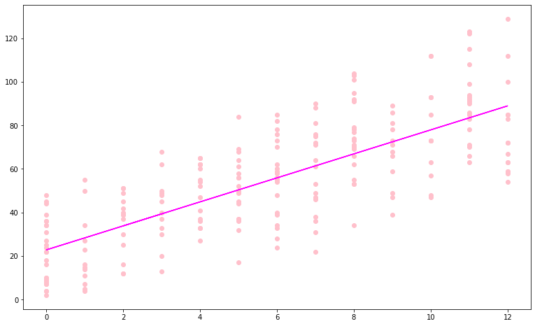
Now we have everything to plot our model:

plt.figure(figsize=(13,8))
plt.scatter(x, y, color = "pink")
plt.plot(x, coef * x + intercept, color = "fuchsia")
plt.show()

Now that we have our model, we can determine if its a good model by verifying these 3 conditions:

• The error shouldn’t be dependent
• The expected value should be around 0
• The residuals should follow normal distribution

We can check the first two condition by plotting the residuals into a scatter plot:

plt.scatter(x, y - (coef * x + intercept), color = "pink")
plt.plot(x, 0 * x, color = "fuchsia")
plt.show()

As we can see, the error isn’t dependent and the expected value seems to be around 0.

We can check the last condition by plotting the residuals into a histogram:

n, bins, patches = plt.hist(y - (coef * x + intercept), bins = 30, color = "pink", density = True)

mue = np.mean(y - (coef * x + intercept))
sigma = np.std(y - (coef * x + intercept))
normd = norm.pdf(bins, mue, sigma)

plt.plot(bins, normd, color = "fuchsia")

plt.show()

The residuals more or less seem to follow normal distribution.

Lastly, to score our model we can use the score function. This function calculates the value known as R2:

print("R2:", model.score(x,y))

R2: 0.5835324959871742

Judging by the 3 conditions and the R2 score we can say that this model in our case isn’t very reliable, but roughly accurate.

Bonus

To predict a value we can use the predict function of our model:

# Predicting 2 and 8 hours
model.predict([[2],[8]])

array([[33.8597135 ],
       [66.91445534]])

Interpretation: Studying 2 hours gets you around 34 points. Studying 8 hours gets you around 67 points.