Simple Logistic Regression using sklearn

Creating logistic regression in python can be intimidating at first, but with some practise it’s easier than you would’ve imagined. First, we need to import some key libraries:

import numpy as np
import pandas as pd
import matplotlib.pyplot as plt

from sklearn import metrics
from sklearn.linear_model import LogisticRegression as lor
from sklearn.model_selection import train_test_split as sp

Now we can import some data with pandas:

data = pd.read_excel("data/grades.xlsx")
data.head()

Next thing we need to do is to change all our categorial variables to numeric values for later use in logistic regression:

data["Bestande"] = data["Bestande"].map({"WHACK":0,"Durchschnitt":1})

Now we can split our data into test and training data and get a quick overview of our data:

train, test = sp(data, test_size = .3)

x = data["Stunden"].values.reshape(-1, 1)
y = data["Bestande"].values

x_train = train["Stunden"].values.reshape(-1, 1)
y_train = train["Bestande"].values

x_test = test["Stunden"].values.reshape(-1, 1)
y_test = test["Bestande"].values

plt.scatter(x, y)

Our data looks like this:

Next up we can create our model with the training data,

model = lor().fit(x_train, y_train)

create predictions

x_predict = np.linspace(0, 12, 20).reshape(-1, 1)
y_predict = model.predict_proba(x_predict)[:,1]

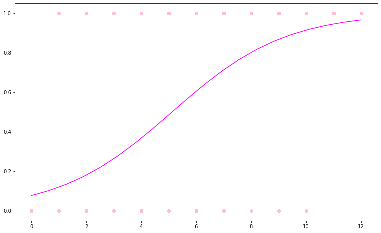
and plot our regression:

plt.figure(figsize=(13,8))
plt.scatter(x, y, color = "pink")
plt.plot(x_predict, y_predict, color = "fuchsia")
plt.show()

With our test data we can score our model. There are 2 ways to do this. The first one is with a confusion matrix:

y_predict_score = model.predict(x_test)

confm = metrics.confusion_matrix(y_test, y_predict_score)
print("confusion matrix:", "\n", confm, "\n")

score = (confm[0][0] + confm[1][1]) / np.sum(confm)
print("score:", score)

confusion matrix: 
 [[21  8]
 [ 4 31]] 

score: 0.8125

The second one is with the score function:

print("score:", model.score(x_test, y_test))

score: 0.8125

Bonus

Like the LinearRegression model, the LogisticRegression model returns coefficient (a) and intercept (b) values.

a = model.coef_
b = model.intercept_

We can use these values to calculate the probability with this mathematic formula:

To predict the probability of a value we can also use the predict_proba function of our model:

# Predicting 2 and 8 hours
model.predict_proba([[2],[8]])

array([[0.81942292, 0.18057708],
       [0.17493011, 0.82506989]])

Interpretation: Studying 2 hours means you have a 82% chance of not approving (y = 0) and a 18% chance of approving (y = 1). Studying 8 hours means you have a 17% chance of not approving and a 83% chance of approving.